Estimating Snow Extent From Sentinel-2 Imagery
This article builds on the previous two (Part-1, Part-2) articles that illustrate the fetching and processing of satellite data that is made available in the COG format. The simplicity of processing satellite imagery when made available in the COG data format, has had me running more quick desktop investigations of which this is one.
Here I was interested in the insight into seasonal variability that could be gained by estimating and comparing snow cover over multiple years.
Disclaimer
This is a lightweight desktop investigation over a small number of seasons. This should not be used to draw any conclusions of trends.
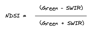
NDSI
For the purpose of delineating snow, the NDSI (Normalized Difference Snow Index) is employed. This detects snow by using the ratio of the difference in the Green and Shortwave Infrared (SWIR) reflectance. This calculation is based on the properties of snow that has high amounts of visible light reflected while absorbing SWIR energy.
The NDSI output values range from -1 to 1 with values greater than 0.42 considered snow ( ESA technical guidlines).
Getting Started
Fetching the Satellite Data
Python functions
The below Python functions for fetching and evaluating the COG data are discussed in Part-1 of this recent series on COGs. For this reason I wont spend time discussing them but point out the few alterations required to calculate NDSI.
Optimising for Cloud Free Images
In the recent COG based investigations we filtered out all scenes with cloud. However, it is expected the more scenes we have over our area of interest, the better insights we will gain into how snow cover develops over each season. For this reason, rather than limiting our search of scenes to near zero percent cloud cover, we accept a degree of cloud cover in each image as long as it is not affecting the extraction of the snow extents. To be sure of this, once we have fetched the imagery we can visually inspect the dataset and remove any scenes that may not be suitable for NDSI calculations.
Of note, while cloud and snow at times can be near impossible to distinguish by the naked eye in satellite imagery, the NDSI is very effective at distinguishing between the two classes and a great tool to use when unsure if viewing snow or cloud.
import matplotlib.pyplot as plt
import matplotlib.animation as animation
import numpy as np
import rasterio
from rasterio.plot import show, reshape_as_image
from pyproj import Transformer
from satsearch import Search
from datetime import datetime

%matplotlib inline

# Sentinel-2 STAC API
url = "https://earth-search.aws.element84.com/v0/"

# The % of cloud tolerated in the area of interest
subset_scene_cloud_tolerance = 25

# Bounding Box delineating the spatial extent for NDSI mapping
bbox = [170.61241369919802, -43.99718122852591, 170.72304010411418, -43.927003638993675]

# The date range for mappinpg NDSI overtime
date_range = "2018-01-01/2021-12-31"
Differing Band Resolutions
While the green band samples the Earth’s surface at a 10 metre resolution, the SWIR data is collected at 2 metres.
As the NDSI formular requires that the calculation is applied across these two bands, we are required to reshape the SWIR band so that it has the same pixel dimensions. This is achieved by resampling. Below when reading the COG data for the SWIR band (Band 11) we apply resampling as outlined in the Rasterio documentation
def range_request(image_url, bbox, bands = 1, resample=False, resample_width=None, resample_height=None):
    """
    Request and read just the required pixels from the COG
    """
    with rasterio.open(image_url) as src:
        coord_transformer = Transformer.from_crs("epsg:4326", src.crs)
        # calculate pixels to be streamed from the COG
        coord_upper_left = coord_transformer.transform(bbox[3], bbox[0])
        coord_lower_right = coord_transformer.transform(bbox[1], bbox[2])
        pixel_upper_left = src.index(coord_upper_left[0], coord_upper_left[1])
        pixel_lower_right = src.index(coord_lower_right[0], coord_lower_right[1])

        # request only the bytes in the window
        window = rasterio.windows.Window.from_slices(
            (pixel_upper_left[0], pixel_lower_right[0]),
            (pixel_upper_left[1], pixel_lower_right[1]),
        )

        # The affine transform - This will allow us to
        # translate pixels coordiantes back to geospatial coordiantes
        transform_window = rasterio.windows.transform(window,src.transform)

        if resample:
            data = src.read(bands,
                out_shape=(
                    src.count,
                    resample_height,
                    resample_width
                ),
                resampling=rasterio.enums.Resampling.bilinear,
                window=window,
            )

        else:
            data = src.read(bands, window=window)
        return(data, transform_window)
Querying STAC API
def image_search(bbox, date_range, scene_cloud_tolerance):
    """
    Using SatSearch find all Sentinel-2 images
    that meet our criteria
    """

    # Note, we are not querying cloud cover and accepting
    # all images irrelevant of cloud metadata.
    search = Search(
        bbox=bbox,
        datetime=date_range,
        collections=["sentinel-s2-l2a-cogs"],
        url=url,
        sort=['<datetime']
    )

    print('%s items' % search.found())
    return search.items()
Calculating Cloud Cover
def percent_cloud_cover(scl):
    """
    Calculate the cloud cover in the subset-scene
    """
    image_size = scl.size
    unique, count = np.unique(scl, return_counts=True)
    counts = dict(zip(unique, count))

    # sum cloud types
    cloud_med_probability = counts.get(8, 0)
    cloud_high_probability = counts.get(9, 0)
    thin_cirrus = counts.get(10, 0)
    total_cloud_cover = cloud_med_probability + cloud_high_probability + thin_cirrus

    # percent subscene cloud cover
    percent_cloud_cover = 100 * float(total_cloud_cover) / float(image_size)
    print(f"\t cloud cover {percent_cloud_cover}%")

    return percent_cloud_cover
Fetch the images and Calculate the NDSI
By employing the functions above:
- Query the STAC API
- Assess the area of interest (as defined by the bounding box) for cloud.
- Request only the imagery within our bounding box for the bands we require
- Calculate the NDSI
- Add the required data to the images list for analysis and visualisation
# The images we are going to estimate snow extents with
images= []

# out of interest we will store cloud cover for all sub-scenes.
# We can then generate stats about cloud for all observations
scene_assessment = {}

# Iterate over all observations meeting our search criteria
items = image_search(bbox, date_range, scene_cloud_tolerance)
for item in items:

    # Refs to images
    green = item.asset("green")["href"]
    swir = item.asset("swir16")["href"]
    rgb = item.asset("visual")["href"]
    scl = item.asset("SCL")["href"]
    date = item.date.strftime("%d/%m/%Y")

    # Calculate cloud cover for the sub-scene
    if subset_scene_cloud_tolerance:
        print(f"Assessing Cloud Cover: {date}")
        scl_subset, transform_window = range_request(scl, bbox)
        cloud_percent = percent_cloud_cover(scl_subset)
        scene_assessment[date] = cloud_percent
        print(f"clouds in subset-scene: {date}")
        if cloud_percent > subset_scene_cloud_tolerance:
            continue

    # Streamed pixels within bbox
    green_subset, transform_window = range_request(green, bbox)

    # The shape of the 10m band will be use for the outsize of the 20m resampling
    ten_meter_shape = green_subset.shape
    swir_subset, transform_window = range_request(swir,
                                                  bbox,
                                                  True,
                                                  1,
                                                  ten_meter_shape[1],
                                                  ten_meter_shape[0])
    rgb_subset, transform_window = range_request(rgb, bbox, [1, 2, 3])

    #Calcualte NDSI
    ndsi_subset = (green_subset.astype(float) - swir_subset.astype(float)) / (
        green_subset + swir_subset
    )

    # Store the data for further processing
    images.append(
        {"date": date,
         "rgb": rgb_subset,
         "ndsi": ndsi_subset,
         "transform_window": transform_window,
         "snow_mask_sieved": None # Storing for visualisation purposes
         "snow": None,
         "snow_area": 0}
    )
Visualise the Image Data
Here we visualise all our images that we have selected for analysis. It is worth noting any images that may have been selected that could have cloud obscuring snow observations.
from matplotlib import gridspec
import matplotlib as mpl

# compute the number of rows and columns
n_plots = len(images)
n_cols = int(np.sqrt(n_plots))
n_rows = int(np.ceil(n_plots / n_cols))

# setup the plot
scale = max(n_cols, n_rows)
fig = plt.figure(figsize=(5 * scale, 5 * scale))
grid = gridspec.GridSpec(n_rows, n_cols, fig, wspace=0.4)

# iterate through each subplot and plot each image
for i in range(n_plots):
    ax = fig.add_subplot(grid[i])
    show(images[i]['rgb'],
                        transform=transform_window,
                        ax=ax,
                        alpha=.65,
                        title = images[i]['date']
                       )

for ax in fig.get_axes():
    ax.ticklabel_format(style ='plain') # show full y-axis labels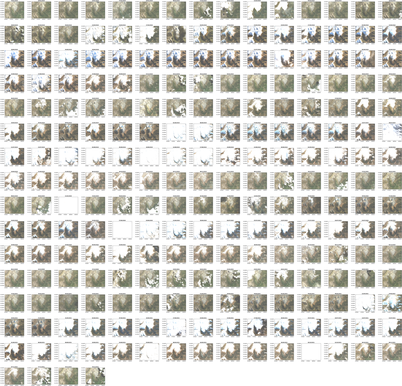
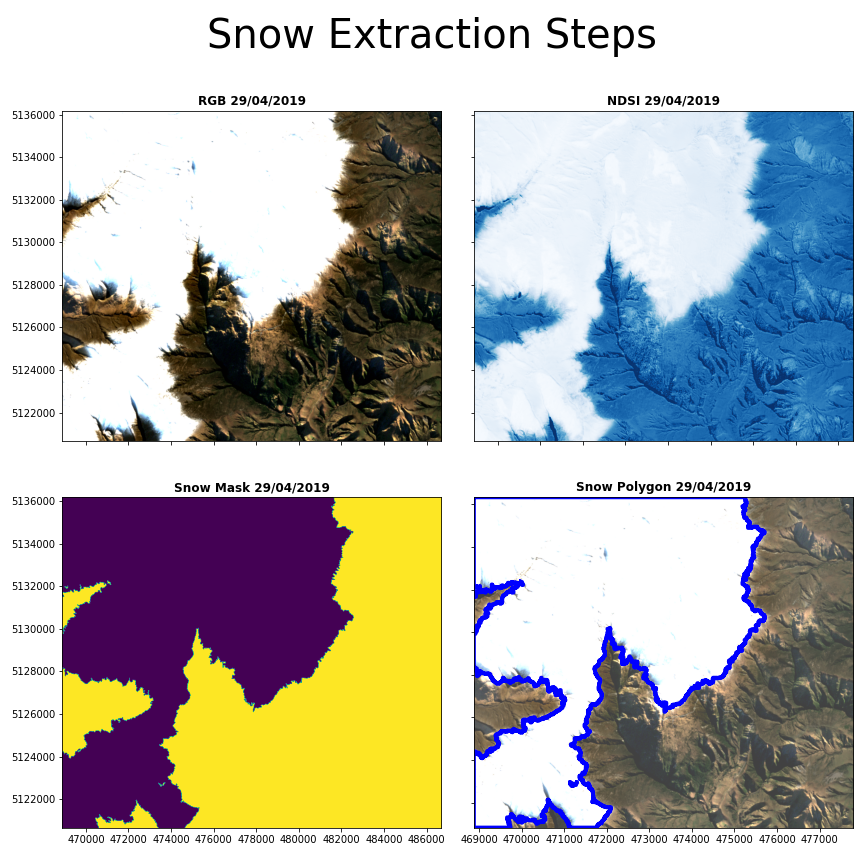
Mask NDSI
Now that we have fetched the required images and calculated the NDSI values for each image, we will extract snow polygons for all NDSI values greater than the threshold for delineating snow. In the case of Sentinel-2, pixels with a NDSI value greater than 0.42 are considered snow (ESA technical guidlines)
By following the below steps we extract the snow polygon extents:
- Use Numpy’s
masked_lessmethod to mask the NDSI values below the 0.42 threshold. - These outputs can have some noise and we apply a sieve to generalise some of this out.
- Turn the mask into polygons via Rasterio
features.shapesmethod - Read the polygons into as Geopandas dataframe
- Once in a dataframe we query this data and return just the polygons that represent snow.
- Using the output from the above, the area of snow cover can be calculated and stored for each image
* *Note, we are calculating the area for a 2d planar surface (as opposed to the real 3d world) and this will under represents true snow area. We are not using these values to determine the exact snow area but as a proxy of snow cover for comparison.
from rasterio import features
import geopandas as gpd
import json
from shapely.geometry import shape

for image in images:

    # Mask out all values below the NDSI threshold (these are not snow)
    # Values above NDSI 0.42 are generally considered snow
    snow_mask = np.ma.masked_less(image['ndsi'], 0.42)

    # Sieve speckle
    snow_mask_sieved = features.sieve(snow_mask.mask.astype('uint8'), 20, out=None, mask=None, connectivity=4)

    # Extract the polygons from the mask
    snow_polygons = rasterio.features.shapes(source=snow_mask_sieved.astype('uint8'),
                                       transform=image['transform_window'],
                                       )

    # Add all polygons to the list
    snow_polygons = list(snow_polygons)

    # Extract the polygon coordinates and values from the list
    polygons = [polygon for polygon, value in snow_polygons]
    values = [str(int(value)) for polygon, value in snow_polygons]

    # Convert polygons into a shapely.shape
    polygons = [shape(polygon) for polygon in polygons]

    # Create a geopandas dataframe populated with the polygon shapes
    snow_geodataframe = gpd.GeoDataFrame({'is_snow': values,
                           'geometry':polygons},
                           crs="EPSG:32759")

    # Dissolve all records into two records. is snow / is not snow
    is_snow = snow_geodataframe.dissolve(by='is_snow')

    # Select only the snow records
    snow = is_snow.query("is_snow=='0'")

    image['snow']=snow
    image['snow_mask_sieved']=snow_mask_sieved
    if len(snow.area) == 1:
        image['area']=snow.area[0]/1000000 # in km2
    else:
        image['area']=0
Visualise the Masks and Snow Polygons
Below are the key steps for our snow area calculations visualised: NDSI, Mask and snow polygons.
Graph Estimated Snow Cover By Year
Format the data by year
As our analysis will take a per annum view, lets format the data required for analysis by year to simplify this process.
Here we also want to filter out images we have identified as being too cloud affected.
# The date of the images we have identified as too cloud affected
not_suitable_for_analysis = [datetime.strptime('21/02/2020', '%d/%m/%Y').date(),
                             datetime.strptime('17/06/2020', '%d/%m/%Y').date(),
                             datetime.strptime('03/10/2021', '%d/%m/%Y').date(),
                             datetime.strptime('16/07/2019', '%d/%m/%Y').date()]

by_year = {}
for image in images:

    date = datetime.strptime(image['date'], "%d/%m/%Y").date()
    day_of_year = date.strftime('%j')
    year = date.year

    # If we have flagged an image after visual inspection as not suitable
    # We will not add it to our data for analysis
    if date in not_suitable_for_analysis:
        continue

    if year not in by_year.keys():
        by_year[year] = {'date' : [], 'area' : [], 'rgb': []}

    by_year[year]['date'].append(date)
    by_year[year]['area'].append(image['area'])
    by_year[year]['rgb'].append(image['rgb'])
Graph Each Observation’s Snow Area by Year
By graphing each observation’s snow area by year, we can compare each seasons snow cover.
As a ski-field is located within our area of interest, we have also added a window (in grey) to each graph indicating the relationship of the ski season with snow cover.
import matplotlib.dates as mdates
import math

# Get the largest area of snow
# this will set the max value of the y axis
max_snow_coverage = max(list([area for area in v['area'] for v in by_year.values()]))
max_snow_coverage = int(math.ceil(max_snow_coverage / 10.0)) * 10

fig, axs = plt.subplots(len(by_year.keys()), figsize=(12,10),  sharey=True)
fig.suptitle('Total area of snow (km²)', fontsize=20)

for ax, year in zip(axs, by_year):
    ax.plot(by_year[year]['date'],
            by_year[year]['area'],
            )
    ax.set_xlim([date(year,1, 1), date(year,12,31)])
    ax.set_ylim([0,max_snow_coverage])

    # Highlight the ski season on the graph
    # dates based on expected season dates for 2022
    ski_seaon_begin = datetime.strptime(f'01/07/{year}', '%d/%m/%Y')
    ski_seaon_end =datetime.strptime(f'25/09/{year}', '%d/%m/%Y')
    ax.axvspan(ski_seaon_begin, ski_seaon_end, facecolor='grey', alpha=0.2)

    if year != list(by_year.keys())[-1]:
        ax.set_xticks([])
    ax.set_title(year)

ax.xaxis.set_major_formatter(mdates.DateFormatter('%d-%b'))
fig.text(0.08, 0.5, 'Total snow area (km²)', va='center', rotation='vertical')
Sanity Check
Image comapre
To sanity check the plotted data, it is useful to plot all images by year with the area displayed prominently. This allows as to visually view the amount of snow present in image and the resulting snow area we calcualted to ensure nothing appears amiss.
for year in by_year.keys():

    # compute the number of rows and columns
    n_plots = len(by_year[year]['rgb'])
    n_cols = int(np.sqrt(n_plots))
    n_rows = int(np.ceil(n_plots / n_cols))

    # setup the plot
    scale = max(n_cols, n_rows)
    fig = plt.figure(figsize=(5 * scale, 5 * scale))
    fig.suptitle(f'\nAquired Cloud Free Images For {year}', fontsize=80)
    grid = gridspec.GridSpec(n_rows, n_cols, fig, wspace=0.4)

    # iterate through each subplot and plot each set of data
    for i in range(n_plots):
        ax = fig.add_subplot(grid[i])
        show(by_year[year]['rgb'][i],
             transform=transform_window,
             ax=ax,
             title = f"{by_year[year]['date'][i]}\n{by_year[year]['area'][i]}km2")
    for ax in fig.get_axes():
        ax.label_outer()
        ax.ticklabel_format(style ='plain') # show full y-coords

    fig.tight_layout()
    fig.savefig(f"{year}_images.png")
    plt.subplots_adjust(left=None, bottom=None, right=None, top=0.9, wspace=None, hspace=0.02)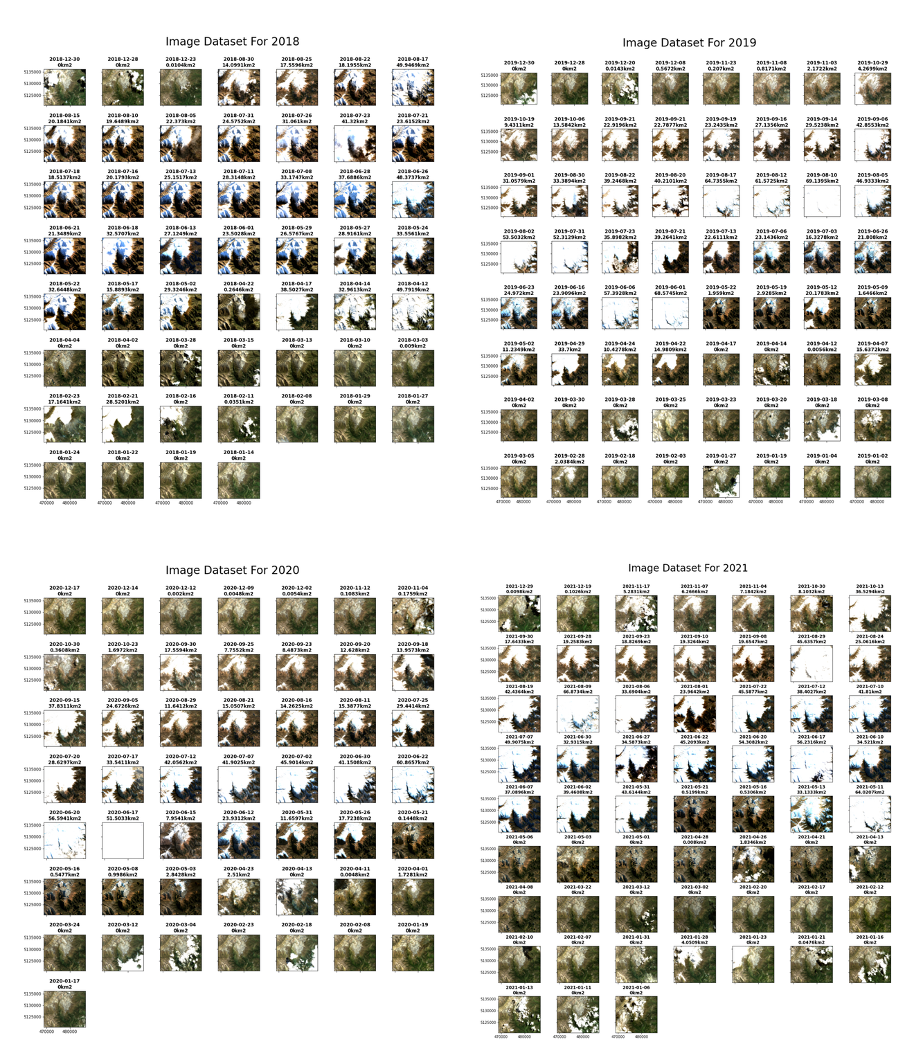
Bonus
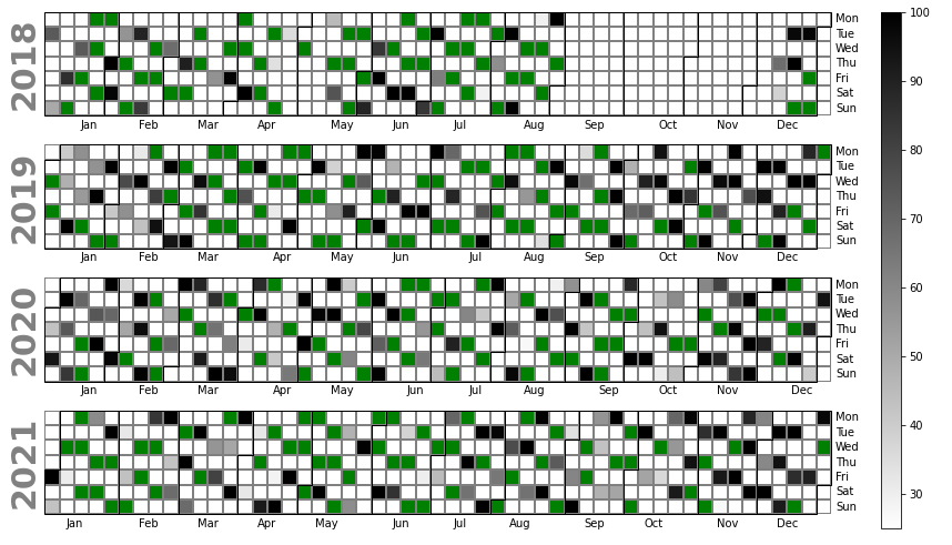
Plotting the data aquisitions
Below all Sentinel-2 data for our investigation period is plotted. The Green data points indicate the data that meet our criteria of being 75% cloud free. The grey data points represent the data which we did not use due to cloud presence and the degree of cloud present.
This turned out the be very useful as it was suspect some data was missing. However the extent of this missing was not made clear until producing the below plot.
This appears to be an issue with the data store and I am investigating further with the intention to raise an issue against this data sotre.
import calplot

obs_dates = [pd.to_datetime(datetime.strptime(date, '%d/%m/%Y').strftime("%Y-%m-%dT%H:%M:%S")) for date in scene_assessment.keys()]
obs_cloud_cover = [cloud_cover for cloud_cover in scene_assessment.values()]

events = pd.Series(obs_cloud_cover, index=obs_dates)
events.index

my_cmap = matplotlib.cm.get_cmap('binary')
my_cmap.set_under('g')
fig = calplot.calplot(events,
                      cmap=my_cmap,
                      colorbar=True,
                      vmin=25,
                      fillcolor='white',
                      linecolor="grey",
                      edgecolor="black" )