Intro

To explore extracting vegetation height from LiDAR data, a swath from the Land-use and Carbon Analysis System (LUCAS) LiDAR data was acquired from the Ministry for the Environment (MFE). This data is ideal for such calculations as its collected in heavily forested areas and is at a resolution high enough to analyse individual trees.

The computation of vegetation height using LiDAR is fairly straightforward.

1. A Digital Surface Model (DSM) must be extracted from the LiDAR point data. This is a model representing features elevated above the “Bare Earth”.
2. A Digital Terrain Model (DTM) must be extracted from the LiDAR point data. This is a Bare Earth model with surface features not included.
3. What is commonly known as a Canopy Height Model (CHM) is then produced by subtracting the DTM from the DSM.

Extracting the DSM and DTM from LiDAR

The PDAL (Point Data Abstraction Library) is a very powerful tool for processing LiDAR point cloud data and very adept at extracting surface models based on point classification and filtering algorithms.

PDAL allows the composition of operations on point clouds into ‘pipelines’. These pipelines are written in the JSON format and define each step for the processing of the data in a sequence. This leads itself to highly customisable point cloud processing, that is repeatable and runs many steps in one execution of the program.

DSM PDAL Pipeline

Below is the pipeline I composed for extracting the DSM from the LiDAR point cloud.

{

    "pipeline":[
        "LEVEL2_24304A_20150414_S004/LEVEL2_24304A_20150414_S004.las",
        {
            "type":"filters.reprojection",
            "in_srs":"EPSG:2193",
            "out_srs":"EPSG:2193"
        },
        {
            "type":"filters.range",
            "limits":"returnnumber[1:1]"
        },

        {
            "type": "writers.gdal",
            "filename":"dsm.tif",
            "output_type":"idw",
            "gdaldriver":"GTiff",
            "resolution": 0.5,
            "radius": 1

        }
    ]
}

Parameters

The PDAL parameters most important to extracting the Surface Model are outlined below

Filter

A filter is applied to filter on the “returnnumber”. To generate a DSM we are only interested in the first returns as these are the LiDAR returns from the highest points measured by each light pulse. These first returns are represented by the returnnumber 1

Writers

The writer defines the parameters for calculating the output and the output data type.

Of use in this case are the below parameters:

• Resolution: Length of raster cell edges in X/Y units.
• Radius: The value where each point that falls within a given radius of each raster cell center contributes to the raster cells value.

DTM PDAL Pipelne

{
    "pipeline":[
         "LEVEL2_24304A_20150414_S004/LEVEL2_24304A_20150414_S004.las",
        {
            "type":"filters.reprojection",
            "in_srs":"EPSG:2193",
            "out_srs":"EPSG:2193"
        },
        {
          "type":"filters.assign",
          "assignment":"Classification[:]=0"
        },
        {
          "type":"filters.elm"
        },
        {
          "type":"filters.outlier"
        },
        {

          "type":"filters.smrf",
          "ignore":"Classification[7:7]",
          "slope":0.2,
          "window":16,
          "threshold":0.45,
          "scalar":1.2
        },
        {
          "type": "writers.gdal",
          "last":true,
          "filename":"dtm.tif",
          "output_type":"idw",
          "gdaldriver":"GTiff",
          "resolution": 0.5,
          "radius": 1
        },
        {
          "type":"filters.range",
          "limits":"Classification[2:2]"
        }
    ]
}

Parameters

The PDAL parameters important to extracting the LiDAR ground returns that represent a DTM are discussed in the following sections.

Classification Values

In this case we want to ignore any LiDAR classification values that may have already been calculated so that we can derive our own. In this example we apply a value of 0 (not classified) to the Classification dimension for every point.

Filter Low Point Outliers

The Extended Local Minimum (ELM) algorithm identifies low points that can adversely affect ground segmentation algorithms. These points are marked as noise with the default ELM noise value of 7 as per the las specification.

Outliers

Used to identify any outlier points that may affect ground segmentation. The filter aims to indicate any points that are statistical outliers due to LiDAR signal noise. Like the outliers identified with ELM these are also classified with a value of 7.

Ground Classification

The filters.smrf classifies ground points based on the well accepted Simple Morphological Filter (SMRF) approach. The points classified as noise (value 7) are filtered out of the final result. Following the LAS format, those points identified as ground are given the classification value of 2.

Ground Return Filter

Having classified ground points by giving such points the classification value of 2, the points are filtered out to create a model solely representing bare ground.

Running the pipelines

Once the steps are defined in the pipeline, it is as simple as running the below commands to build the models

pdal pipeline dxm_pipeline.json

Calculating the CHM

Once the DSM and DTM models have are computed, GDAL can be used to run a raster calculator to output the CHM.

gdal_calc.py -A dtm.tif -B dsm.tif --calc="B-A" --outfile chm.tif

Visualising the CHM model via Python and matplotlib

As a means to visualise the CHM, Python along with Matplotlib was used. This method of visualisation was selected, as with one script a well annotated map can be generated in a format that is ready to include in documents such as reports and in this case, a website.

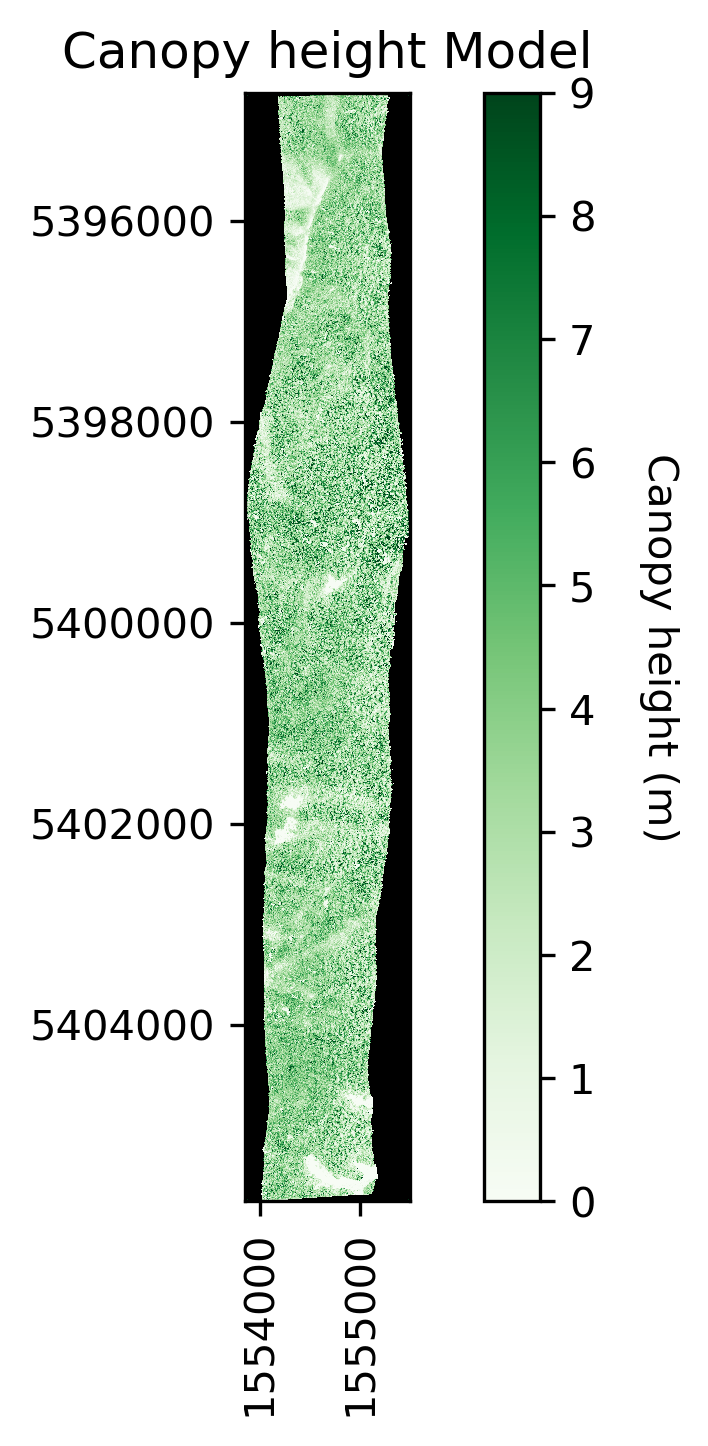
Below, the Python code for generating the CHM visualization.

import numpy as np
import os
import gdal, osr
import matplotlib.pyplot as plt
import sys


def plot_band_array(
    band_array, image_extent, title, cmap_title, colormap, colormap_limits
):
    plt.imshow(band_array, extent=image_extent)
    cbar = plt.colorbar()
    plt.set_cmap(colormap)
    plt.clim(colormap_limits)
    cbar.set_label(cmap_title, rotation=270, labelpad=20)
    plt.title(title)
    ax = plt.gca()
    ax.ticklabel_format(useOffset=False, style="plain")
    rotatexlabels = plt.setp(ax.get_xticklabels(), rotation=90)


chm_file = "/home/splanzer/git/chm/chm.tif"


# Get info from chm file for outputting results
just_chm_file = os.path.basename(chm_file)
just_chm_file_split = just_chm_file.split(sep="_")

# Open the CHM file with GDAL
chm_dataset = gdal.Open(chm_file)

# Get the raster band object
chm_raster = chm_dataset.GetRasterBand(1)

# Get the NO DATA value
noDataVal_chm = chm_raster.GetNoDataValue()

# Get required metadata from CHM file
cols_chm = chm_dataset.RasterXSize
rows_chm = chm_dataset.RasterYSize
bands_chm = chm_dataset.RasterCount
mapinfo_chm = chm_dataset.GetGeoTransform()
xMin = mapinfo_chm[0]
yMax = mapinfo_chm[3]
xMax = xMin + chm_dataset.RasterXSize / mapinfo_chm[1]
yMin = yMax + chm_dataset.RasterYSize / mapinfo_chm[5]
image_extent = (xMin, xMax, yMin, yMax)


# Plot the original CHM
plt.figure(1)
chm_array = chm_raster.ReadAsArray(0, 0, cols_chm, rows_chm).astype(np.float)

# Plot the CHM figure
plot_band_array(
    chm_array,
    image_extent,
    "Canopy height Model",
    "Canopy height (m)",
    "Greens",
    [0, 9],
)
plt.savefig(
    "/home/splanzer/git/chm/CHM.png",
    dpi=300,
    orientation="landscape",
    bbox_inches="tight",
    pad_inches=0.1,
)