1. Introduction

To understand the impacts of widely predicted sea-level change and coastal inundation, a seamless surface model of both the land topography and underwater bathymetry is required (NOAA, 2007). However, due to how data for these models is traditionally captured, there is a data gap between the surface models that prevents the joining of the land and seafloor surfaces.

Modern topographic surface models are derived from airborne topographic LiDAR (Light Detection and Ranging) data. Topographic LiDAR data collection employs active sensors most commonly emitting energy at 1,064nm. While these sensors are very effective at mapping the land’s surface, they do not penetrate the water column to allow overlap between land and sea data collection. Modern bathymetric mapping employs shipborne sonar sensors. While very effective at mapping the seafloor surface, it is impossible to acquire bathymetric data in the nearshore as the depths do not allow operation of a ship. This paper investigates the suitability of Satellite Derived Bathymetry (SDB) to predict water depths in inshore zones for filling the data gap between the land and sea surfaces.

2. Methodology

2.1. Study Area

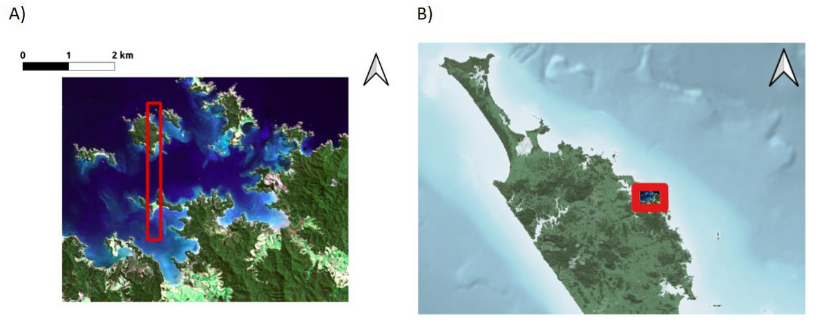
The study area is in the Bay of Islands, New Zealand (Figure 1). The coastal morphology is of mainland and island coastlines comprising of exposed rock out crops broken by sandy beaches. There are also small estuarine systems within the study area and large estuaries bordering its boundary that are sources of sediment and localised turbid water. The area is approximately 120km2 (10x12km), though is of approximately a 50% ratio of land to water. Water depth ranges from 0m to ~28m.

The study area is split into two areas of unequal size. The smaller of the two is for calibration of the SDB and the larger extent, to test the extrapolation of SDB outside of the area where in-situ measurements were collected for the SDB calibration. This tests two concepts: 1) How accurate is SDB with calibration points spread throughout the area? and 2) Can a strip of random measurements be taken for a small subset of the scene, SDB coefficients calculated from these and then applied to the entire scene saving time and money by requiring less in-situ measurements?

2.2. Data

2.2.1. Multibeam echosounder data

Multibeam echosounder (multibeam) is currently the most accurate method for measuring water depths (Chénier et al., 2018). In this study the multibeam data is used to calibrate the SDB model as well as assess the accuracy of the SDB depths.

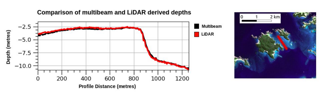
The multibeam data was captured in 2010 as part of the Oceans 2020 project. Multibeam data should be captured as close as possible to the satellite image acquisition date to ensure that the nature of the seafloor has not change between the period the multibeam survey and the satellite imagery was collected. This is especially important in dynamic regions. To be sure that the multibeam’s acquisition age was suitable for comparison to Sentinel-2 products (not operational until June 2015) the multibeam data was compared to a marine LiDAR derived surface from 2013 and the seafloor was deemed to be stable (see Figure 2). The LiDAR was not used for calibration and assessment as it was of a relatively small area and incomplete.

2.2.2 Satellite Imagery

2.2.2.1. Scene Selection

It is important that there is no cloud cover over the study area, minimal water turbidity, nor any signs of sun glint caused by reflection from the slope of waves present when the scene was capture. This criterion quickly ruled out most scenes. Swell was assessed by visual inspection and its lack thereof was also checked by analysing the waters response to NIR, based on the assumption that NIR should be absorbed by water and any variation in NIR values is due to sun glint. To find an image meeting all the above criteria, close to two years of imagery was discarded before a suitable image was found from Sentinel-2A from March 5th, 2017. This image was corrected to L1C prior to download, meaning that it was geometrically corrected by DEM and radiometrically corrected to Top of Atmosphere.

2.2.2.2. Atmospheric Corrections

As part of this investigation, the effectiveness of applying atmospheric corrections to the Sentinel-2A L1C image was tested. This is due to the fact that a literature review revealed little consensus as to the validity of correcting for atmospheric effects for SDB. For example, Monteys et al. (2015) stated “Several studies focusing on measuring water quality using Landsat sensors have questioned the advantage of using atmospherically corrected data when attempting to describe the variability of optical water properties” (Monteys et al., 2015).

Atmospheric corrections were applied using the ACOLITE processor (https://github.com/acolite/acolite) developed specifically for aquatic remote sensing applications. The ACOLITE processor was configured to use Dark Spectrum Fitting which allows for the estimation of an atmospheric path that is relatively insensitive to sun glint (RBINS, 2019), a significant issue for SDB.

ACOLITE can also be configured to output parameters derived from the correction algorithm. For the purpose of this investigation the turbidity product using the Dogliott turbidity algorithm was output. This was useful in assessing the study area for SDB suitability and understanding any effects of turbidity on the results.

2.3. Satellite Derived Bathymetry Method

There are many methods for calculating water depths from satellite data. For the purposes of this investigation an empirical approach has been selected. Empirical approaches derive depth by measuring the varying degree to which different bands are attenuated by the water column and apply a regression between in-situ depth measurements and measured attenuation differences. An empirical approach was selected as only satellite data comprising of bands that can penetrate water sufficiently are required. This is opposed to other methods that require seafloor type and water constituent data.

2.3.1. Spatial filtering

Saga GIS simple filter was used to filter out “speckle noise”. This was applied to the blue, green and NIR bands of both the L1C and L2A scenes using a kernel size of 3x3.

2.3.2. Log Ratio Algorithm for Satellite Derived Bathymetry

One of the most widely used formula for calculating SDB is the natural logarithm of the blue band divided by the natural logarithm of the green band (Chénier et al., 2018)

SDB Algorithm Value = Ln (Blue) / Ln (Green)

The algorithm was developed by Stumpf et al. (2003) and is based on the principle that as depth increases the reflectance from the bands will decrease until a point at which contributions from bottom reflectance are no longer detectable. The band of higher absorbance decreases proportionately faster than the band of lower absorbance. Therefore, the ratio between the green and blue bands declines linearly with depth when they are log transformed. (Stumpf et al., 2003). Different water types affect the ratio to which the blue and green bands penetrate the water. In clear water with low organic matter, blue light is attenuated at lower rates than green. While the inverse is true for water with high concentrations of organic matter whereby green light penetrates deeper (Chénier et al., 2019).

2.3.3. Calibrating SDB algorithm values to depths

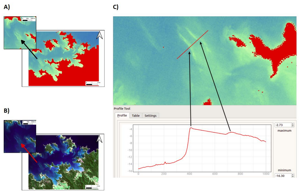
QGIS was used to apply the Stumpf et al. (2003) log ratio formula to every water pixel within the study area for the Sentinel-2A L1C and L2A corrected scenes (Figure 3 shows a subset of the SDB algorithm values mapped in pseudo-colour) Once the SDB algorithm values were calculated for all water pixels, a mathematical correlation between these values and the in-situ multibeam depth measurements needed to be found. To do this, within the calibration area, 10 percent of the pixels with SDB algorithm values associated were randomly selected along with the multibeam depth measurements that were spatially associated to these pixels (Figure 4 indicates the distribution of these calibration measurements). The SDB algorithm values and associated multibeam depth measurements were then imported to a database and by aggregating all unique multibeam depth values along with the SDB algorithm values, the average SDB algorithm value was found for each distinct depth (as measured to two decimal places) within the calibration area for both the L1C and L2A image.

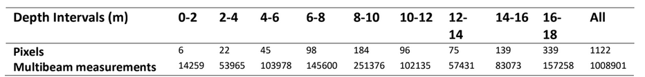
The resulting average SDB algorithm values for each depth were then plotted via scatter plot to investigate if a mathematical correlation existed (see figure 5). From each scatter plot, the extinction depth, that depth at which light from the most attenuated band is not returned and the correlation breaks down, can be determined. In the study area, this showed that depths were still predicted by SDB at the study’s maximum depths. It however also indicated there was no correlation between the SDB algorithm values and measured depths for 0 to 2.15m of water. Reviewing figure 2, it is clear this is due to a lack of calibration data for this depth interval. As a result, for this study SDB depths could not be generated for depths above 2.15m. As the study is focused on the nearshore, the study’s upper-bounds were limited to 18m.

An order 2 polynomial regression coefficient and a coefficient of determination (R²) was calculated for depths between 2.15-18m. It was however found that by dividing the data into 2.15-4m and 4-18m ranges, two regression coefficients (one for each depth interval) fit the data better and more accurately predicted depth from the SDB algorithm values. Using the SDB algorithm values, the appropriate polynomial regression coefficients were applied to every water pixel for the two images (L1C and L2A) to derive depths from the SDB algorithm values.

3. Results

3.1. Calibration area SDB accuracy assessment

10 percent of the pixels and the multibeam depths associated with them were used to calibrate the SDB depth values. The multibeam measurements associated with the remaining 90% of pixels were used for the accuracy assessment by comparing the SDB derived depths to the multibeam measured depths for both the L1C and L2A images within the calibration area.

Error was calculated for each Seintinel-2 pixel that the SDB depths were attached to by subtracting the associated multibeam measured depths. The error calculated for each multibeam measurement was then used to statistically analysis each SDB pixel’s depth. As each pixel is 10x10m, but represents a seafloor that varies in depth, it should be noted some of this calculated error is derived from this issue of spatial resolution. The error statistics do however describe how well each measured multibeam depth is represented by the SDB depths.

Figure 6 shows the SDB errors aggregated by 2 metre depth intervals. For the L1C corrected image, SDB predicted depths accurately for depths 2.15-4 metres with a mean error of -0.189, where negative values indicate SDB over-estimated depth. Depths in the ranges of 8-10m and 10-12m were most poorly predicted by SDB with a mean error of –2.89 and -2.67 (see figure 7). It was initially expected that this would be correlated to a smaller subset of calibration measurements, however figure 3 shows this is not the case. It is therefore proposed the poorer performance for these depth ranges is due to varying bottom types not captured in the calibration data.

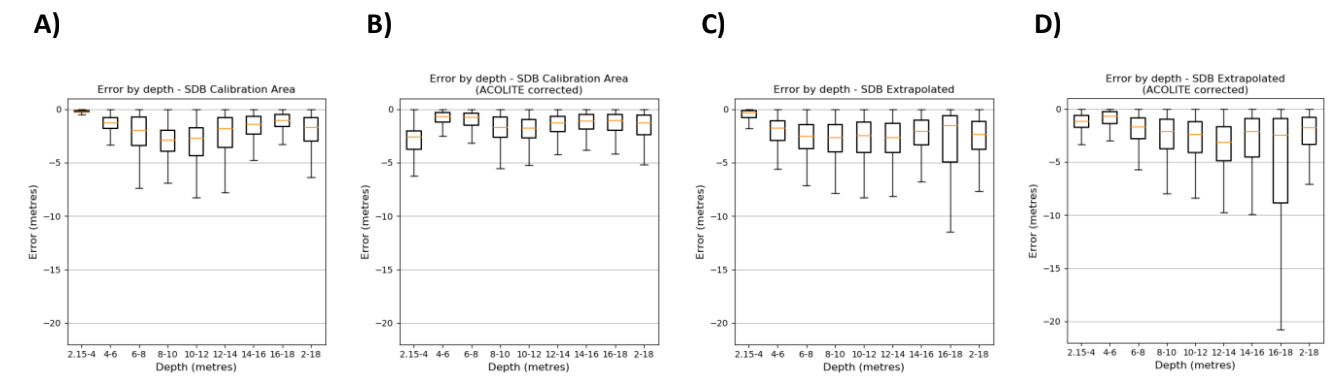
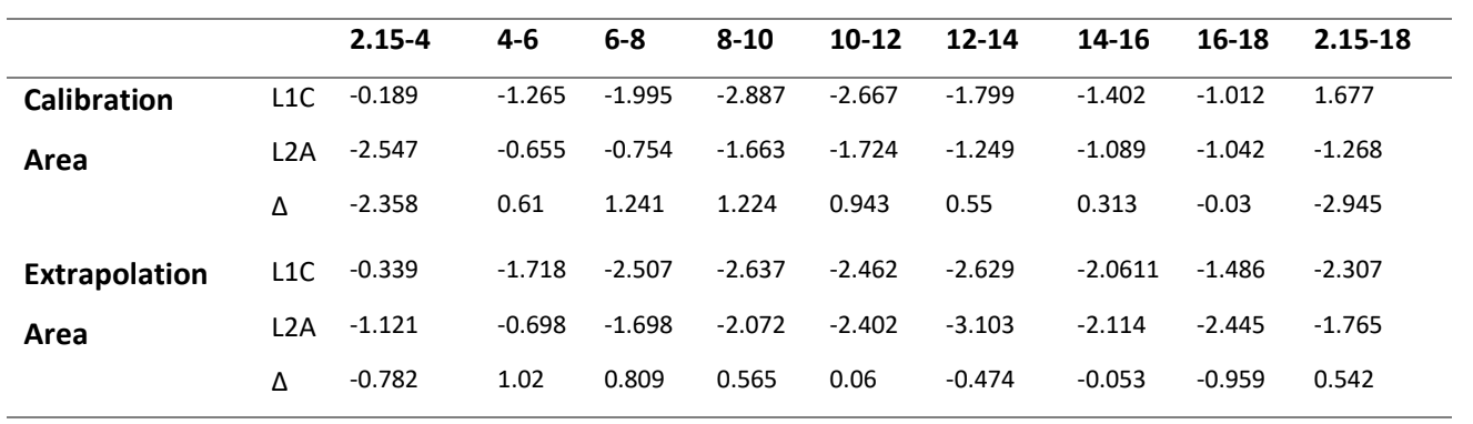
Overall the mean error for the L1C image was –1.667m, and -1.268 for the L2A image. However, the overall mean error for L2A is largely skewed as the L2A correction introduced significant error to depths of 2.15-4m. This introduction of error by using the L2A corrected image is not understood and would require more research to draw conclusions. Overall the atmospheric corrections by ACOLLITE improved SDB depth prediction.

3.2. Extrapolation area SDB accuracy assessment

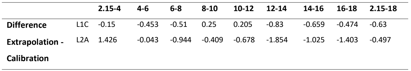
By using the polynomial regression coefficients generated in the calibration area and applying them to the rest of the study area, SDB depth predictions became less accurate. As figure 8 shows, L1C SDB depths outside of the calibration area are 0.63m less accurate and the L2A SDB generated depths are 0.497m less accurate when extrapolated.

3.3. Discussion

It was found that the methodology of deriving SDB outlined in this paper was not suitable in waters of 0 to 2.15m of depth. Shallower depths were of most interest to this investigation as this is where shipborne multibeam cannot operate. It is expected that the SDB depths could not be derived for these shallow waters due to insufficient multibeam measurements in the calibration area for these depths to calibrate the model. It is proposed that to solve this, marine LiDAR where available is used to supplement the multibeam measurements for shallow waters to increase the number of calibration measurement for these depths.

For the depths SDB was calculated for, while the results are not accurate enough for safety of life application such as marine charts, they do have the potential to provide coarse surface models were multibeam surveys do not exist. In many regions only sparse point soundings are available. These soundings could be used to calibrate a SDB surface model that is of finer resolution than what is currently available.

This investigation has demonstrated that atmospheric corrections improve the accuracy of SDB’s ability to predict depths. However, more research is required to understand why error was introduced in the 2.15-4m range.

As a next step it would be useful to use the turbidity output from ACOLITE to investigate the impact of turbidity on SDB.

5. References

NOAA. 2007. Topographic and Bathymetric Data Considerations: Datums, Datum Conversion Techniques, and Data Integration. Part II of A Roadmap to a Seamless Topobathy Surface: National Oceanic and Atmospheric Administration.

Chénier R, Faucher M and Ahola R. Satellite-Derived Bathymetry for Improving Canadian Hydrographic Service Charts. ISPRS Int. J. Geo-Inf. 2018, 7, 306.

Monteys X, Harris P, Caloca S and Cahalane C. Spatial prediction of coastal bathymetry based on multispectral satellite imagery and multibeam data. Remote Sensing 2015, 7, 13782–13806.

RBINS (Royal Belgian Institute of Natural Sciences). ACOLITE Python User Manual (QV - March 26, 2019), https://odnature.naturalsciences.be/downloads/remsem/acolite/acolite_manual_20190326.0.pdf 2019.

Stumpf R.P, Holderied K and Sinclair M. Determination of water depth with high‐resolution satellite imagery over variable bottom types Limnology and Oceanography., 48 (1part2) (2003), pp. 547-556 L2A – D)